To get sensor data, we decided to generate our own by putting sensors into our office. We found Tinkerforge’s system of bricks and bricklets quite nice and easy to start with, so we went for that option.
We got the following four sensor bricklets:
- Sound intensity (basically a small microphone)
- Temperature
- A multi-touch bricklet (12 self-made touch pads from aluminium foil can be connected)
- A motion detector
The four bricklets are connected to a master bricklet, which is in turn connected to a Raspberry Pi.
We put the temperature sensor into a central place in the office. We set up the motion detector in the hallway leading to the kitchen and the bathrooms. We put the sound intensity sensor next to the kitchen door and placed touch sensors on the coffee machine, the fridge door and the door handle for the men’s bathroom.
Although this is clearly a toy setup (and you will have to wait a long time for the data to become big) we quickly came upon some key issues that also arise in real-world situations with sensors involved.
As a storage solution we chose MongoDB, mainly because it was also used in the customer project that motivated the lab.
The data generated by the four sensors can be grouped into two categories: While the temperature and sound intensity sensors output a constant stream of data, the motion detector and multi-touch sensor are triggered by events that typically don’t occur with a fixed frequency.
This gave rise to two different document models in MongoDB. For the first category (streaming), we used the model that MongoDB actually suggests as best practice for such a situation and that could be called the “Time Series Model” (seehttp://blog.mongodb.org/post/65517193370/schema-design-for-time-series-data-in-mongodb). It consists of one collection with nested documents in it. The number of nesting levels and the number of subdocuments on each level depends on the time granularity of the data. In our case, the highest time resolution of the Tinkerforge sensors is 100 ms, which gives rise to the following document structure:
- One document per hour
- Fields: timestamp of the hour, sensor type, values
- Values: nested set of subdocuments: 60 subdocuments for each minute, 60 subdocs for each second, 10 subdocs for each tenth of a second
github:07c69eb8066fcc26f45f
The documents are pre-allocated in MongoDB, initalizing all data fields to a value that is outside the range of the sensor data. This is done to avoid constantly growing documents which MongoDB would have to keep moving around on disk.
Data of the second type (event-driven/triggered) is stored in a “bucket”-like document model. For each sensor type, a number of documents with a fixed number of entries for the values (a bucket of size of e.g. 100) are pre-allocated. Events are then written into these documents as they occur. Each event corresponds to a subdocument which sits in an array with 100 entries. The subdocument carries the start and end time of the event as well as its duration. As the first record/event is written into the document, the overall document gets a timestamp corresponding to the start date/time. On each write to the database, the application checks whether the current record is the last fitting into the current document. If so, it sets the end date/time of the document and starts directing writes to the next document.
github:5540b9939751b3503dbb
These two document models represent the edge cases of a trade-off that seems to be quite common with sensor data.
The “Time Series” model suggested by MongoDB is great for efficient writing and has the advantage of having a nice, consistent schema: every document corresponds to a natural unit of time (in our case, one hour), which makes managing and retrieving data quite comfortable. Furthermore, the “current” document to write to can easily be inferred from the current time, so the application doesn’t have to keep track of it.
The nested structure allows for the easy aggregation of data at different levels of granularity – although you have to put up with the fact that these aggregations will have to be done “by hand” in your application. This is due to the fact that in this document model there are no single keys for “minute”, “second” and “millisecond”. Instead, every minute, second and millisecond has its own key.
This model has issues as soon as the data can be sparse. This is obviously the case for the data coming from the motion and multi-touch sensors: There is just no natural frequency for this data since events can happen at any time. For the Time Series document model this would mean that a certain fraction of the document fields would never be touched, which obviously is a waste of disk space.
Sparse data can also arise in situations where the sensor data does not seem to be event-driven at first. Namely, many sensors, although they measure data with a fixed frequency, only automatically output this data if the value has changed compared to the last measurement. This is a challenge one has to deal with. If one wanted to stick with the time series document model, one would have to constantly check whether values were omitted by the sensor and update the corresponding slots in the database with the last value that was sent from the sensor. Of course, this would introduce lots of redundancy in the database.
The bucket model avoids this by filling documents only with data that have actually been recorded. But it also has its disadvantages:
- If the full data is to be reconstructed afterwards (including redundant data that hasn’t been saved), the application has to handle it
- There is no consistent start and end time for a “bucket” document – if you’re interested in a particular time range, you would have to look up all documents covering this range
- The management of the “buckets” (keeping track of current bucket, checking when it is full) needs to be taken care of by the application
The Tinkerforge sensors come with APIs for a number of languages. We decided on using Python and running the scripts on a Raspberry Pi with the sensors hooked onto it. The data is written to a MongoDB instance hosted on MongoSoup, our MongoDB-as-a-Service solution. To register e.g. the sound intensity and temperature bricklets via the API, you do the following:
github:200a496c9e8e6bdd962a
The Tinkerforge API supports automated reading of data from the sensors via callback functions. To use this feature, you register the function you want to be triggered with the bricklets like this:
github:12dca499fe8f9f4b0064
This will automatically query the sensors for new data every 100 ms and call the functions stream_handler.cb_intensity_SI and stream_handler.cb_temperature, respectively.
The catch here is that in order to save network bandwidth, the functions you supply are only triggered if the measurement of the sensor has changed since the last call – exactly the situation leading to sparse data discussed above.
One could avoid this behaviour by querying the sensor with a fixed frequency directly from custom code. But, as discussed above, this would lead to the database being filled with redundant values. Apart from that, it increases the network overhead from the sensors to the application.
In the end, one will have to decide which model suits the use case better. MongoDB offers a lot of flexibilty regarding the data model, and the choice you settle with should be dictated entirely by the use case, i.e. the most likely read/write patterns you’ll encounter.
A good idea would be to do research before deciding on a document model, asking the following questions:
- From an overall point of view (taking into account database and application performance), is it more expensive to put up with sparsity/redundancy in the database or to reconstruct the redundant data in the application later on?
- How much variance do the data actually have? If periods of constant measurements are relatively rare, then putting up with some degree of redundancy might not hurt too much.
- Are there constant frequencies at a larger timescale? For instance, if your data are basically piecewise constant over periods of a couple of seconds, but these periods are all about the same length, you might consider coarse-graining your time scale and throw away the redundant information from the micro-scale.
- If, on the other hand, the length of the constant varies wildly, then you’re basically in the regime of events happening randomly and would probably be better off with the “bucket” model
In our case, the starting hypothesis was that the temperature and sound intensity data would have sufficient variance to justify storing them in the “Time series” data model, while the motion and touch sensor data would be suitable for the bucket model. This is how we went about.
After completing the setup and implementing the Python scripts handling the sensor data, we started collecting data.
Using matplotlib and the Flask micro-webserver framework, we put up a small web service that visualizes recently collected data for inspection and deployed it to Heroku.

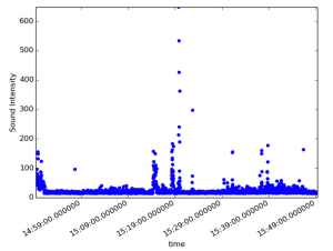
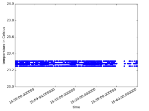
We generated three plots. The first shows events from the touch and motion sensors over time, together with their respective durations. The other two show the levels of sound intensity and temperature over time. Each data point in the plot is calculated by averaging over one second.
A first glance shows the obvious correlation between data from the different sensors caused by human activity in the office.
What you can also conclude is that it was the right choice to use the bucket model for the event data, since there can easily be periods of up to 20 minutes where the sensors don’t record anything.
Looking at the temperature data, it is quite obvious that temperature stays within a range of merely fractions of one degree Celsius, although it does fluctuate substantially on this small scale. If the use case is just to monitor global changes of the temperature during the day, then one could well either coarse-grain the timescale on which data is written or switch to the bucket model altogether.
The sound intensity data is characterised by relatively long periods of very small values, followed by sudden, very short bursts of loud events. One surely doesn’t want to lose this information, so the coarse-graining approach mentioned above is not an option. One could however consider switching to the bucket model and only write data to the database once the measured value changes, if the redundancy introduced by the time-series model gets unacceptable.
Next we’ll perform statistical analysis and pattern recognition on our data and extend the visualisation functionalities. Check back for more on this blog!
Check out part two: https://comsysto.com/blog-post/processing-and-analysing-sensor-data-part-2